Are Discrete Diffusion Models Better Than Auto-regressive Models in Text Generation? Uncovering a Hidden Numerical Issue

Introduction

In this section, we provide a brief and intuitive overview of both continuous and discrete score-based diffusion models. We recommend referring to Yang Song’s blog and Aaron Lou’s blog for more in-depth explanations.

Likelihood-based probabilistic generative modelsTypical likelihood-based models include autoregressive models, normalizing flow models, energy-based models, and variational auto-encoders. Diffusion models, both continuous and discrete, are also likelihood-based. parameterize a density network p_\theta to learn the data distribution p_{\text{data}}. The data space \mathcal X can be either continuous (like \mathbb R^d) or discrete (like \mathcal V^d for vocabulary \mathcal V), where we use d to denote the data dimension. The model can be trained by maximizing the log-likelihood \mathbb E_{x \sim p_{\text{data}}} \left[ \log p_\theta(x) \right], and samples can be generated by drawing from p_\theta.

Training p_\theta faces two major challenges:

• p_\theta must be normalized over all states, i.e., \int_{\mathcal X}p_\theta(x)\mathrm d x=1 (for continuous data) or \sum_{x\in\mathcal X} p_\theta(x)=1 (for discrete data). The former involves an intractable integral, and the latter involves a total number |\mathcal V|^d of states exponential to the data dimension.
• High-dimensional data distributions are typically sparse and hard to fit (curse of dimensionality).

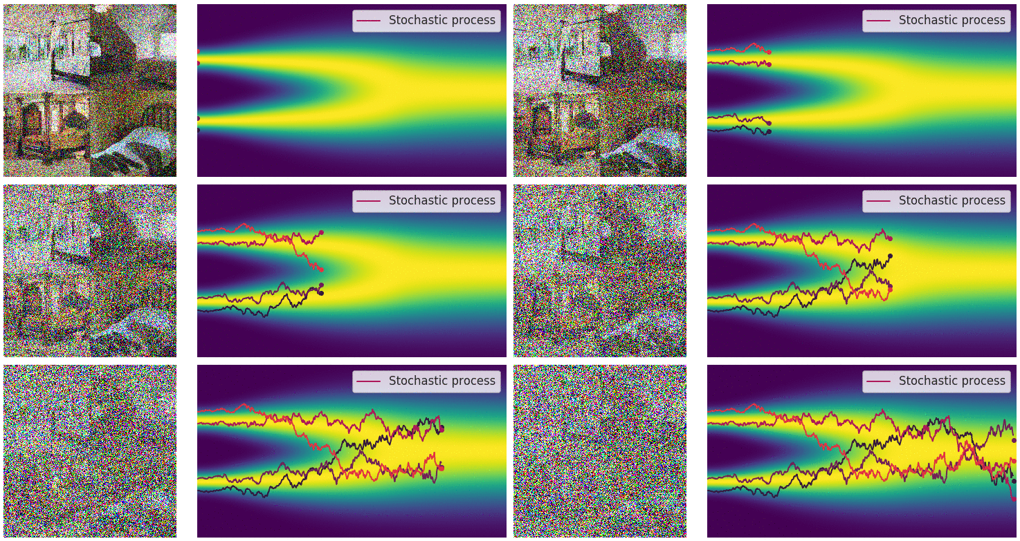
Score-based diffusion models address the first challenge by learning the score function \nabla_x\log p_{\text{data}}(x) which cancels out the normalizing constant, and address the second challange by modeling a series of noise-perturbed distributions \{p_t\}_{t\in[0,1]}. In the continuous-time limit, the forward diffusion process can be described as a stochastic process, with the final distribution being approximately Gaussian, making both learning and sampling manageable. After learning the time-dependent score \nabla_x\log p_t(x), the forward diffusion process can be reversed to approximately draw samples from the data distribution.

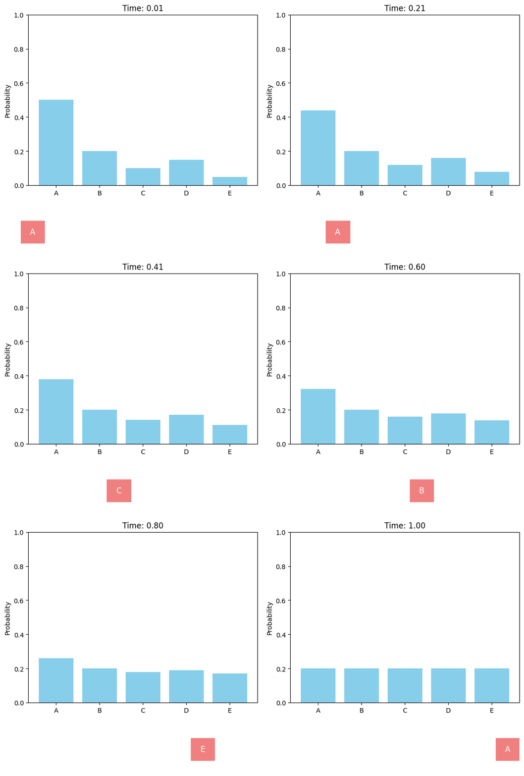
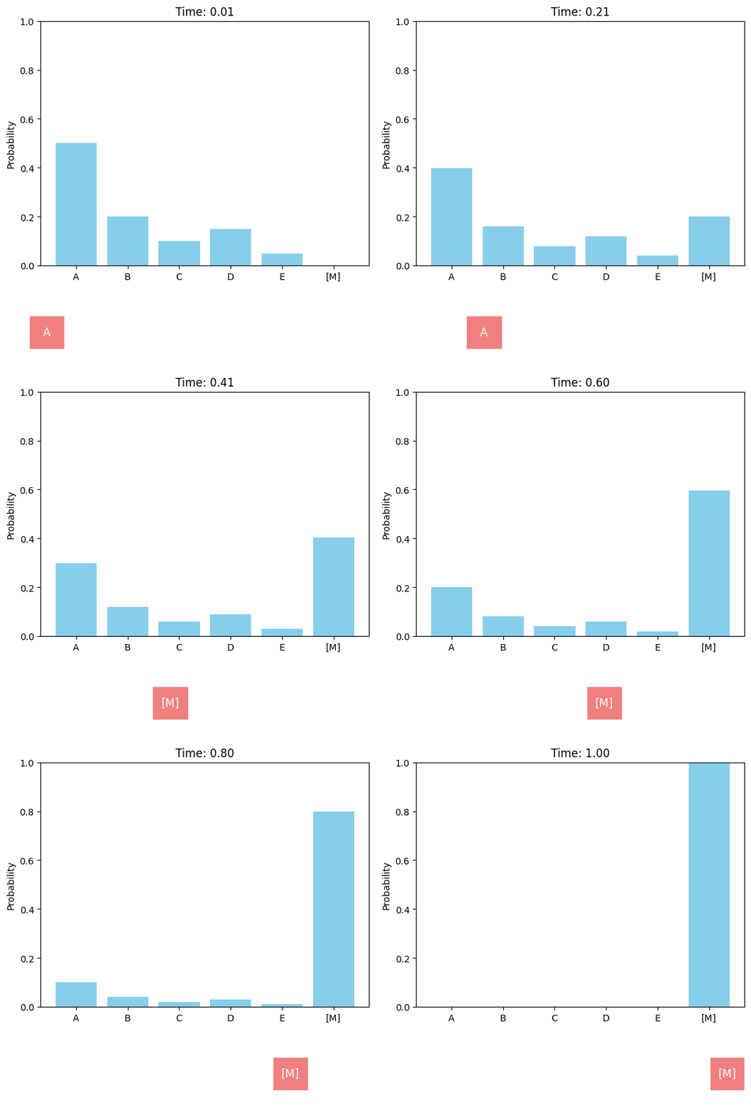
Discrete diffusion models can be defined in a similar score-based continuous-time approach. For the case of single dimension (d=1), the forward discrete diffusion process is described by a continuous-time Markov chain (CTMC), where the token randomly transits according to some predefined rate matrix Q_t. The evolution of the marginal distribution p_t of the token x_t at time t follows the Kolmogorov forward equation \frac{\mathrm d p_t}{\mathrm d t}= p_t Q_t. The forward process can be chosen as uniform or absorbing (or masked), so that p_t converges to a uniform stationary distribution or a concentration on an additionally added mask token [M].

In contrast to the continuous case, the score function \nabla_x\log p_t(x) is not applicable as there is no proper gradient in the discrete space. Instead, the model can learn the probability ratio \frac{p_t(y)}{p_t(x)} between different tokens x and y, which is known as concrete score and also eliminates the normalizing constant. Recently, SEDD proposes the score entropy as a scalable and robust objective for learning the concrete score. With the learned concrete score, the discrete forward process can also be approximately reversed for sampling.

In the multi-dimensional case (d>1), the number of possible states |\mathcal V|^d grows exponentially with the data dimension (e.g., 50527^{1024} for sequences of length 1024 using GPT-2 tokenizer), and it is computationally intractable to model transitions between two arbitrary states. Instead, the model only predicts probabilities of single-token change. Besides, both the forward and reverse processes are factorized across dimensions, where all dimensions undergo transitions simultaneously and independently (except that the network is conditional on all dimensions).

Masked Diffusion Models as the Best-Performing Discrete Diffusion

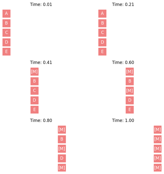
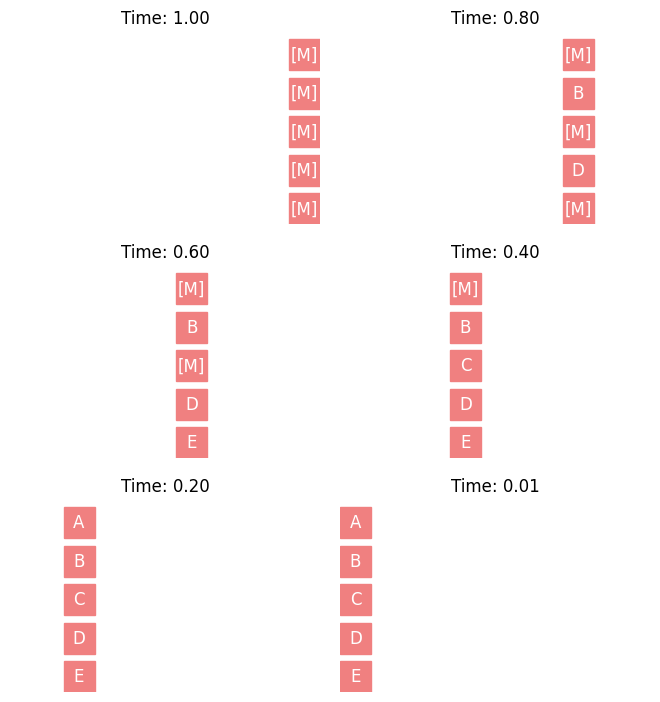
Empirically, the absorbing (or masked) variant demonstrates superior performance over other discrete diffusion schedules such as uniform, and is referred to as masked diffusion models (MDMs). This can be attributed to the simple masked mechanism: transitions are sparse and only happen once between data tokens and the mask token [M] in the whole generation process, which are relatively easier to predict. In some recent works, the masked diffusion formulation is further simplified to a mean-prediction model \mu_\theta with simple weighted cross-entropy training objectives, bringing empirical improvements.

Under mean-parameterization, MDMs become quite similar to typical masked modelsMasked models can be applied to both representation learning (such as BERT, MAE) and generative modeling (such as Mask-Predict, MaskGIT) that learn to reconstruct masked tokens. The key difference is that, MDMs utilize network architectures, training objectives and sampling procedures that rely on the continuous time variable. We illustrate the sampling step in MDMs as follows:

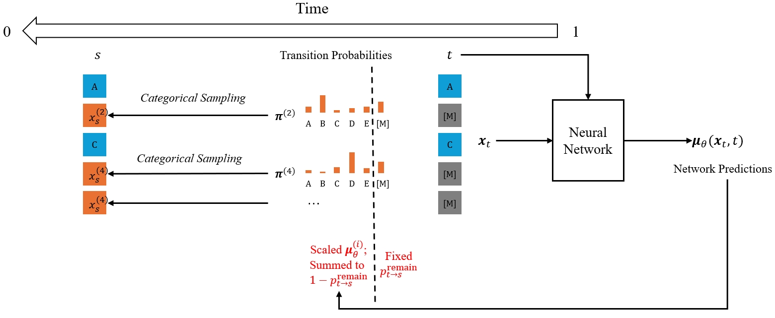
Specifically, let \mathbf x_t=x_t^{(1)}x_t^{(2)}\cdots x_t^{(d)} represent the sequence at time t. For each position i satisfying x_t^{(i)}=\text{[M]}, the transition from time t to time s<t is performed by sampling x_s^{(i)}\sim\text{Cat}(\pi^{(i)}), where \text{Cat} denotes the categorical distribution and \mathbf{\pi}^{(i)}=p_{t\rightarrow s}^{\text{remain}}\mathbf e_{\text{[M]}}+(1-p_{t\rightarrow s}^{\text{remain}})\mu_\theta^{(i)}. Here, \mathbf e_{\text{[M]}} denotes the one-hot vector for the mask token, and the remaining probability p_{t\rightarrow s}^{\text{remain}} is independent of the network output \mu_\theta. In each sampling step of MDMs, whether a masked token will be unmasked is determined by rolling a dice (i.e., categorical sampling), which is distinguished from the token-by-token decoding process of masked models. The number of sampling steps in MDMs can be larger than the sequence length d, and a single sampling step can result in no token changes.

Does Lower Generative Perplexity Indicate Better Quality?

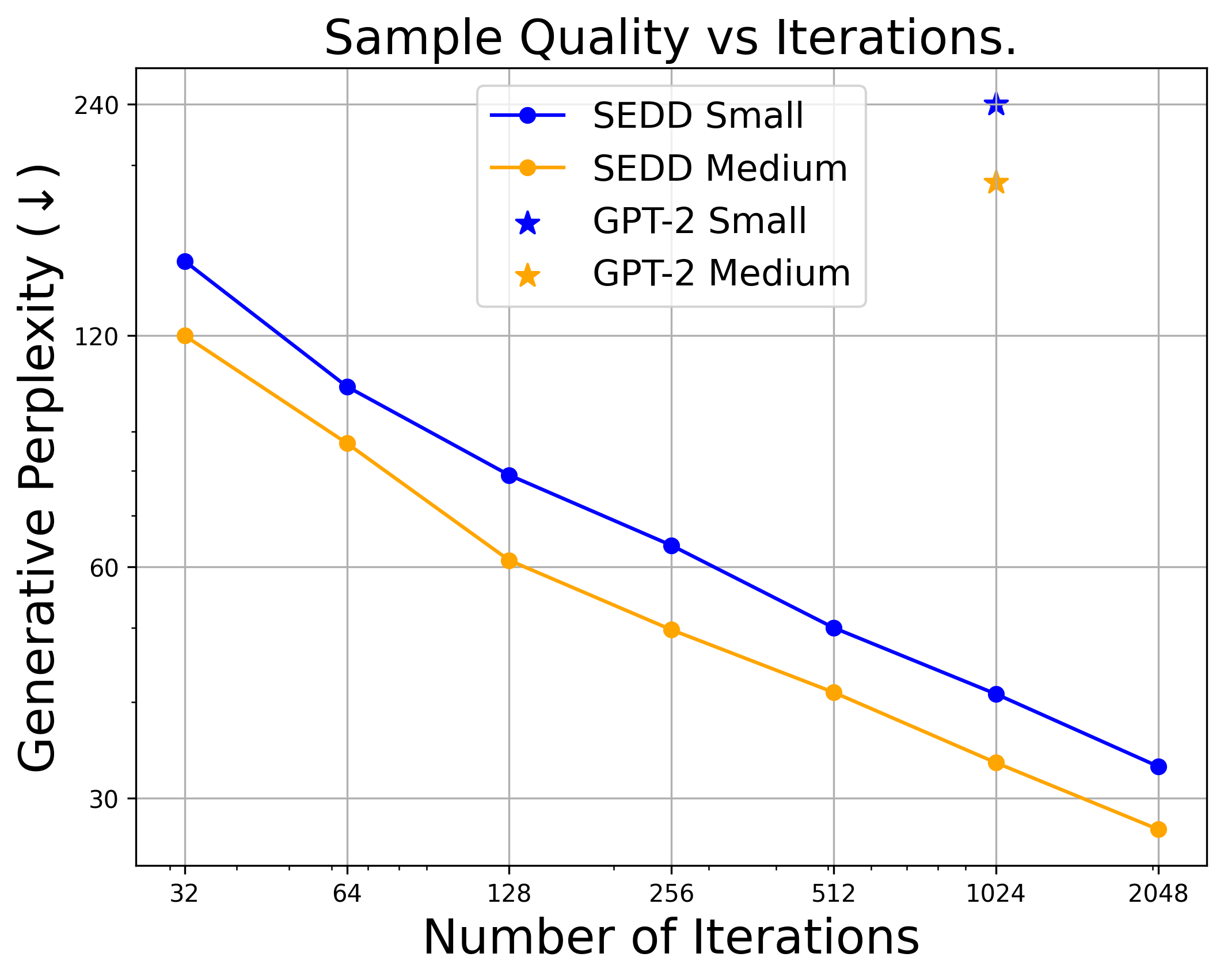
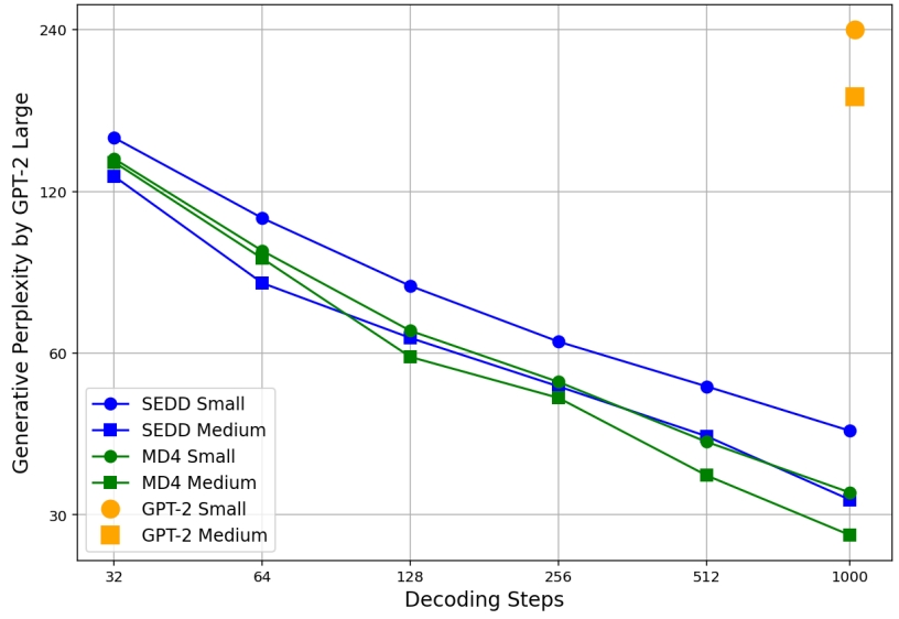
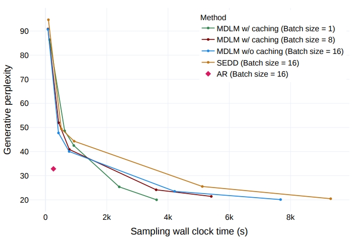
Generative perplexity (Gen PPL) is the main metric in previous works to evaluate the generation quality. Specifically, it measures the likelihood of generated text under some off-the-shelf model (typically GPT-2 Large). Lower Gen PPL means larger probability of the generated sample.

As suggested by multiple previous works, it can be observed that the Gen PPL continues to decrease as the number of sampling steps increases. When the number of sampling steps reaches around 2,000, the Gen PPL of MDMs can even surpass that of counterpart auto-regressive models (ARMs). At first glance, this seems reasonable, as the trade-off between sample quality and inference speed is a key characteristic of diffusion models.

However, we argue that Gen PPL is not comprehensive for evaluating the generation quality of text. Unlike the Fréchet inception distance (FID) metric for images, which compares the whole distribution of generated images with that of real images, Gen PPL only favors high-probability samples, while neglecting other features like diversity and mode coverage.

Token Diversity Matters

We present two samples from ARMs and MDMs to demonstrate the diversity problem.

<|endoftext|> the new cars are crossovers.

AT&T Insurance Marketing Manager, Megan Maxwell, tells us that Model X was "reasonably priced, effective and inspires strong sentiment among consumers." She says:

Our GM car for discussion is shown as part of our drive 20 percent around the world and even a competitor. Our GM for discussion alt shows as one of our most popular cars in the world. We are in multiple countries introducing firmware for our new vehicles. While we are confident in our prices, we rely upon GM Auto’s sales data and know we must adapt this process to meet the needs of all customers.

The proposed pricing is similar to that of the cheaper Range Rover and other cheaper sport utility vehicles, which are primarily offered through its dealerships. Alongside a Volt, Delphi XE8 includes a plug-in hybrid version called Volt Energy.

"Dynamic pricing is our way to deliver owners of more attractive or more reasonable outcomes or to find more marketable models that appeal to them more than their competitors," notes Maxwell.

Earlier this week, GM analyst Greg Clifford predicted that Intel Global Radical Charge Power Savings (STB) would start at $3,300 over the product lifecycle with an adoption rate of 50 percent by 2025.<|endoftext|>

<|endoftext|> I was striking out, he got it to the third out. I know it wasn’t really a catch there, but he didn’t consider that at all. I knew what it wasn’t about. We scored by one run, so it was a difficult thing for me to go to a “get-out,” but being on the board is not an easy fact. I knew it was in play, and went to the third out that it needed to be thrown to. I had nothing to say about it, and it was the only opportunity for me to get, to make an appeal that might not come back, and it was the only time he saw that at that moment.

And so we continued.

“So we were sitting in the plus-five-and-plus-three-at-night, because we were up on an inning. We were in pinch-hit early in the ninth. I looked at a guy and was very nervous and confused, so when I looked at this man — I can’t remember what he was doing, but to double or dead-se the bases for sure — I said you’ll be the first one up, then I’m out of the ballpark. I felt like something had to be wrong with me, and he turned to me and told me, “that’s as bad as the rest,” just like that — “I bet!” I said calmly. “I bet,’” “Gotta do your best! Do not bet!’” “And when that happens, do you think I can be won by a one or two runs?” He stood there and looked stunned. “You mean that?” “Yes, absolutely.” “‘Yeah, absolutely.” “Well, is that a message to you?’“” And he looked back to me and said, “So we aren’t going out?” “Well, yes,” said me, “but I believe so I believe.”” “I bet,” “Yeah, I bet, but when we’re on the board, how much time are we gonna lose?” “Absolutely not,” “I bet,” “all right. I’m not going out. It’s me, understand.” “I bet, I believe not.” “What happened?”” “It happened!” “Did you hear a clue?” “I said, “Oh, no! I-I-I heard that fifth-dinger! Give me the clue!” The players, myself, and the “Man, Man, Man, it’s just beyond hell!” murmurs of the players. At the same time, I said, myself, “Young man, I’ve got to say — I won’t screw you right here.” I went on, “You can take it. You’re not going to lose.”” I smiled. “You know what you got to admit to yourself? This happened in baseball. I didn’t screw you in baseball, it don’t matter, I’ll screw you in a way.” He took the fifth-dinger and said, “It’s the end in baseball, it’s the end.” “That’s correct!” I said. “Yes, you can’t win in baseball,” I said. “But you’re not winning in baseball.” He turned to me. “No, really, it’s alright whether you’re winning or not.” — “I’m sure,” he said. “Good money!” — I cut off. “You’re not going to get this out. You do.” Those were a few words. As I were thinking, “What an enterprise.”

“What are you in baseball?”

“Ah, and it’s a game, not a story and a number. If you believe the most in-the-30s stories are about the when-they-had-to-be-done-as-cardinals-but-recan’t-they-get-in story?” I said “suck,” and “We did stop listening to the number, and we had to come off with the number.”

“Exactly,” said Mike. <|endoftext|>

With as many as 50,000 sample steps, MDMs can reach an extremely low Gen PPL. However, repetitive patterns such as “I bet!” and “I said” frequently appear, diminishing the diversity of tokens in the sequence.

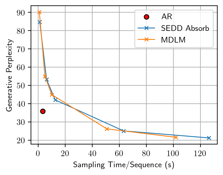
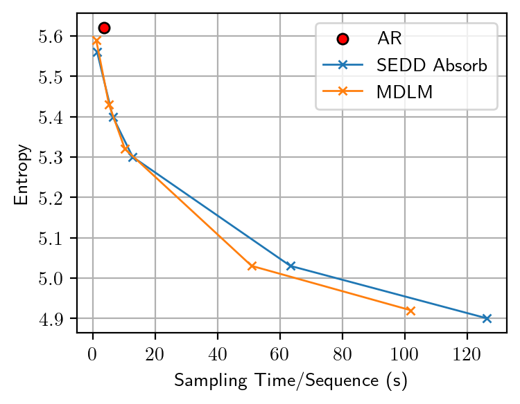
To quantitatively assess the token diversity, we additionally measure the sentence entropyFor a sequence of length L that contains K distinct tokens, with each token k occurring L_k times, the entropy is computed as -\sum_{k=1}^K p_k \log p_k, where p_k = L_k/L represents the probability of occurrence of token k.. We find that the entropy of MDMs, both in the absorbing case of SEDD and in its later improved version MDLM, is consistently lower than that of ARMs and continues to decrease with more sampling steps.

Trade-Off between Generative Perplexity and Entropy

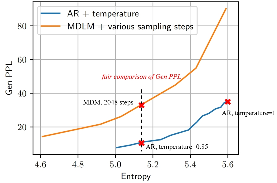
Our observations reveal that varying the number of sampling steps in MDMs creates an inherent trade-off between Gen PPL and entropy. This effectively changes the temperature, leading to an unfair comparison with ARMs, which are not subject to temperature scaling. After manually adjusting the temperature for ARMs to ensure a fair comparison at the same entropy level, we find that the Gen PPL of MDMs falls significantly behind.

What is the Root Cause of Reduced Diversity?

The reduced token diversity and low generation quality is unexpected. In theory, increasing the number of sampling steps should reduce discretization errors and more accurately reflect the true model performance, as already seen in continuous diffusion models. We therefore consider this an implementation issue and investigate further to identify the root cause.

Identifying the Numerical Precision Issue

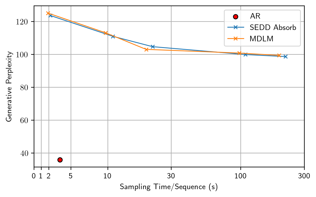
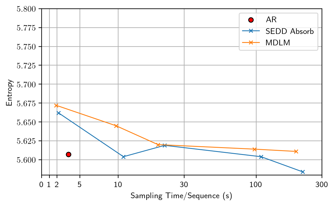
Surprisingly, we find that by simply altering the floating-point precision during sampling from 32-bit to 64-bit, the entropy returns to a normal level similar to ARMs (5.6~5.7), but with a generative perplexity \approx100. After careful ablations, we identify the root cause as the numerical inaccuracy in previous Gumbel-based categorical sampling.

Denote \mathcal U(0,1) as the uniform distribution on [0,1], and \mathcal G(0,1) as the standard Gumbel distributionhttps://en.wikipedia.org/wiki/Gumbel_distribution. To sample from a categorical distribution with class probabilities \pi=[\pi_1\ \pi_2\ \cdots\ \pi_K], Gumbel-max trickAn introduction to the Gumbel-max trick can be found at https://homes.cs.washington.edu/~ewein//blog/2022/03/04/gumbel-max/. is used by first sampling K independent uniform variables u_i\sim\mathcal U(0,1), then transforming them into samples from \mathcal G(0,1) by g_i=-\log(-\log u_i), and finally obtaining the categorical sample n=\arg\max_{i} (\log\pi_i+g_i).

The operation g=-\log(-\log u) theoretically maps u\in[0,1] to g\in(-\infty,+\infty). But due to the limited representation ability of floating-point numbers in implementation, u is constrained to [0,1-\epsilon] and g is constrained to (-\infty,M] where M=-\log(-\log (1-\epsilon))For a floating-point format where the fraction part has f bits, \epsilon can be calculated as 2^{-f-1}. For example, the 32-bit floating point precision corresponds to f=23,1-\epsilon\approx 0.9999999404,M\approx 16.6355.. Therefore, the sample g instead follows a truncated Gumbel distribution, denoted \mathcal T \mathcal G(0,1,M), which refers to the Gumbel distribution \mathcal G(0,1) conditioned on g\leq M. This tricky difference theoretically makes the categorical sampling inaccurate, i.e., \arg\max_{i} (\log\pi_i+g_i) no longer follows the class probabilities \pi.

To verify that truncation is the fundamental issue, we conduct ablations by only modifying the categorical sampling code. We manually scale 64-bit uniform samples to match the truncation in the 32-bit case. We then randomly generate 8 samples with 2048 steps and compare the average Gen PPL and entropy.

For both Gen PPL and entropy, 32-bit\approx64-bit + truncation, which confirms the impact of truncation.

Theoretical Explanations

Through further derivation, we are surprised to find that the effect of truncation can be precisely described in closed-form. Specifically, suppose the original class probabilities are sorted as \pi_1\leq\pi_2\leq\cdots\leq\pi_K. With the truncated Gumbel distribution \mathcal T\mathcal G(0,1,M), the resulting categorical samples instead follow shifted class probabilities \pi ':

To the best of knowledge, such formulations are revealed for the first time by us.

This has two main implications:

• As \beta(i)\geq 0 and \pi_n are sorted, if \pi_{n_1}>\pi_{n_2}, the adjusted class probabilities satisfy \frac{\pi_{n_1}'}{\pi_{n_2}'}>\frac{\pi_{n_1}}{\pi_{n_2}}. This indicates that relatively larger probabilities are further amplified. Therefore, for each position in the sequence, the resulting categorical distribution is biased towards classes with higher probabilities, creating an effect similar to lowering the temperature.
• As \pi include the probability of remaining as [M], different network outputs lead to varying shifting effects, resulting in unequal remaining probability for masked tokens at different positions. Therefore, some mask tokens are prioritized to be unmasked, thereby reducing randomness.

Both factors reduce the diversity and lower the entropy. However, we find that 32-bit categorical sampling produces similar results to 64-bit in token-by-token decoding procedures of ARMs and masked models, suggesting that the first factor is relatively insignificant. In contrast, the distinctive reverse-time sampling procedure of MDMs also suffers from prioritized unmasking. The temperature-lowering effects accumulate across numerous sampling steps, eventually leading to notable diversity issues, even under 32-bit floating-point precision.

Concluding Remarks

In this blog, we illustate how previous works on masked diffusion models secretely suffer from numerical precision issues, leading to somewhat unfair evaluations and doubtful claims. This blog is partially from our paper on arXiv, where we additionally prove that masked diffusion models are exactly equivalent to masked models in both training and sampling, except for some minor aspects like the loss weighting. Our investigation suggests:

• Generative perplexity alone cannot comprehensively reflect the text generation quality. In practice, it better to use the trade-off curve between generative perplexity and sentence entropy for a more holistic evaluation.
• Masked diffusion models are essentially performing maximum likelihood training of masked models. According to our practice, masked diffusion models, along with other discrete diffusion variants, are far from beating the auto-regressive paradigm in text generation.

Despite our negative findings, we acknowledge that the text-based experiments may inherently favor ARMs, as text naturally follows a left-to-right order that ARMs are better suited to model. Recent works on masked modeling of images suggest that the masked mechanism could offer advantages over autoregressive next-token prediction in other modalities. In such cases, maximum likelihood training is often unnecessary for achieving good generation quality, and we can directly use masked models like MaskGIT instead of discrete diffusion models, as they are equivalent to the best discrete diffusion variant while offering simpler formulations.